When Bigger Models Stop Helping: A Practical Demo of the Bayes Error Floor

Imagine you’re building a model to predict whether a patient has a disease based on their symptoms. After going through the full pipeline — data cleaning, feature engineering, modeling — you reach an accuracy of 83%.

In a stakeholder meeting, you confidently say:

“We can probably push this to 90%.”

Then the real work begins.

You tune hyperparameters.

You try more data.

You switch to bigger, more powerful models.

But nothing changes. The accuracy barely moves.

And then it hits you:

Two patients can have identical symptoms…

and still have different diagnoses.

At that point, a different kind of question emerges:

What if the problem itself has a limit?

There’s a Third Possibility

When a model stops improving, we usually assume one of two things:

• The model isn’t powerful enough
• The training process isn’t good enough

So we respond accordingly:

• Try a deeper model
• Tune hyperparameters
• Add more data

But there’s a third possibility that is often overlooked:

The data itself does not contain enough information.

Even with the perfect model, trained perfectly, some predictions would still be wrong. Not because the model failed — but because the problem is inherently ambiguous.

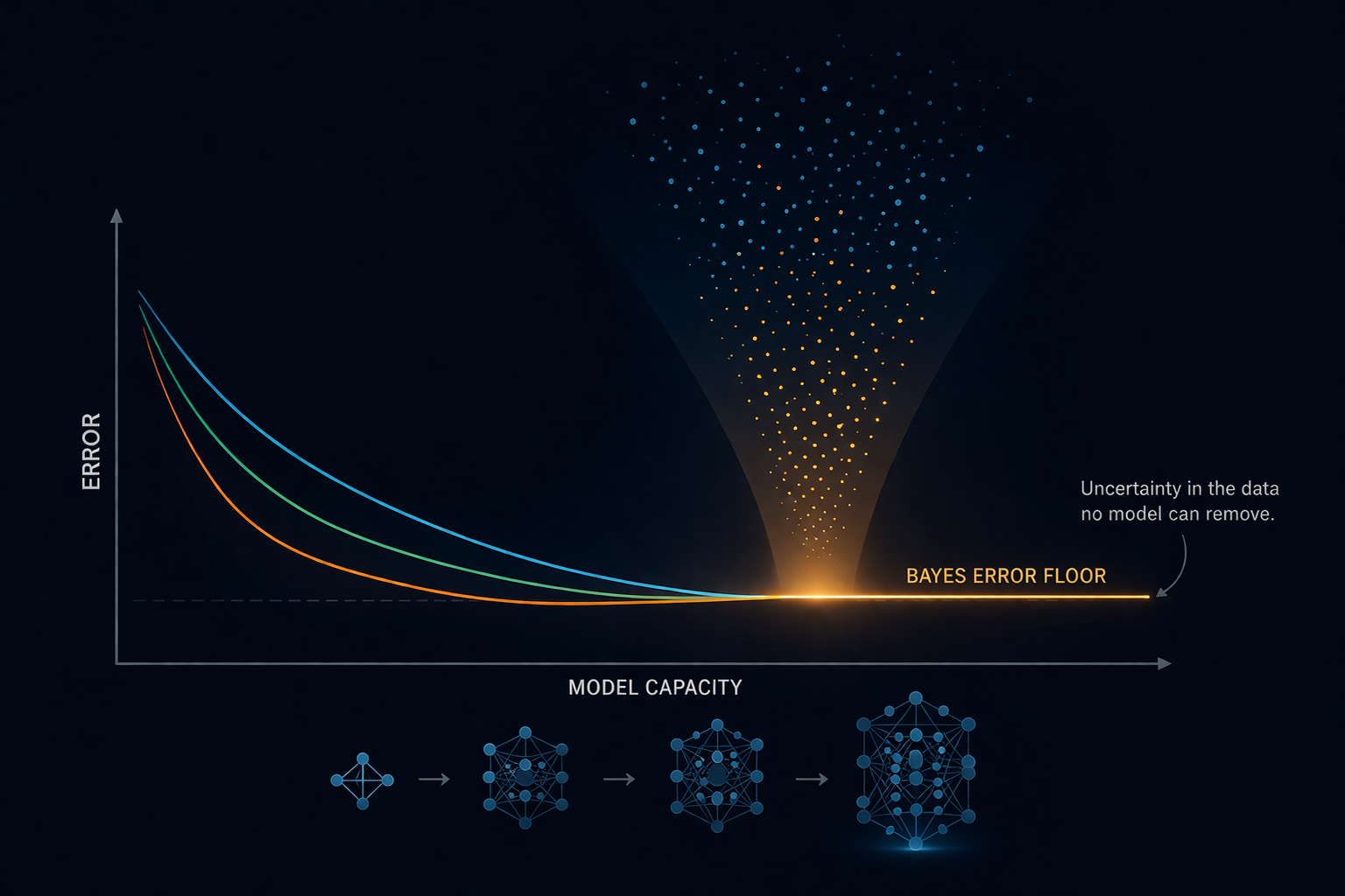
The Bayes Error (and Why it Matters)

This unavoidable uncertainty has a name:

Bayes Error.

It represents the lowest possible error any model can achieve on a given problem.

Not because models are limited —

but because the data itself is.

In simple terms:

Even if you had the perfect model, you still wouldn’t get everything right.

Why?

Because sometimes, the same input can legitimately map to different outcomes.

Bayes Error Through the Lens of Information Theory

Machine learning is often described as learning a function from inputs to outputs. But another useful way to think about it is this:

Machine learning is about reducing uncertainty using the information available in the data.

Before seeing any features, the label has some inherent unpredictability. In information theory, this is captured by Entropy — a measure of how uncertain the outcome is before you know anything. Once we observe the features, some of that uncertainty is reduced. How much uncertainty was removed is captured by Mutual Information — the overlap between what the features tell you and what the label is.

But features rarely explain everything completely. The uncertainty that remains after observing the inputs is captured by Conditional Entropy — H(Y|X). This is the part of the label’s unpredictability that the features simply cannot explain.

And this is exactly where Bayes Error lives.

In our experiment with 20% label noise, the features still perfectly separate the two classes — X > 0 predicts the true label without error. But 20% of the labels were randomly flipped, so the features no longer predict the observed label perfectly. That 20% is pure conditional entropy. It is uncertainty that no model can resolve, because it has no structure, no pattern, and no feature that explains it. It is just noise.

In practice, Bayes Error is tied to this remaining uncertainty — the part of the problem the features simply cannot explain. A model can only do as well as the information in the features allows. Everything beyond that is irreducible.

Let’s Make This Concrete

To see this in action, we’ll create a simple dataset where:

• The true relationship is known
• We deliberately introduce uncertainty

This allows us to control how much information is available — and observe what happens when that information is limited.

Step 1: Create a dataset with controlled noise

import numpy as np
from sklearn.model_selection import train_test_split

np.random.seed(0)

n = 20000

# Input feature
X = np.random.randn(n, 1)

# True rule: perfectly predictable
y = (X[:, 0] > 0).astype(int)

# Inject irreducible noise
noise_rate = 0.2

flip = np.random.rand(n) < noise_rate
y[flip] = 1 - y[flip]

# Split data
X_train, X_test, y_train, y_test = train_test_split(X, y)

The underlying rule here is simple:

• If X > 0 → class 1
• Else → class 0

A perfect model could achieve 100% accuracy. So, we introduce noise. 20% of labels are randomly flipped. This means that even a perfect model cannot exceed 80% accuracy and that 20% is pure uncertainty. It cannot be learned, no matter what model we use.

Step 2: Try increasingly powerful models

from sklearn.metrics import accuracy_score
from sklearn.linear_model import LogisticRegression
from sklearn.neural_network import MLPClassifier

models = {
    "Logistic Regression": LogisticRegression(),
    "MLP (small)": MLPClassifier(hidden_layer_sizes=(10,), max_iter=2000),
    "MLP (large)": MLPClassifier(hidden_layer_sizes=(100, 100), max_iter=2000),
}

for name, model in models.items():
    model.fit(X_train, y_train)

    train_acc = accuracy_score(y_train, model.predict(X_train))
    test_acc = accuracy_score(y_test, model.predict(X_test))

    print(f"{name} → Train: {train_acc:.3f}, Test: {test_acc:.3f}")

We try models with increasing capacity:

• A simple linear model
• A small neural network
• A much larger neural network

If model capacity was the limiting factor, we should see accuracy improve. But that’s not what happens.

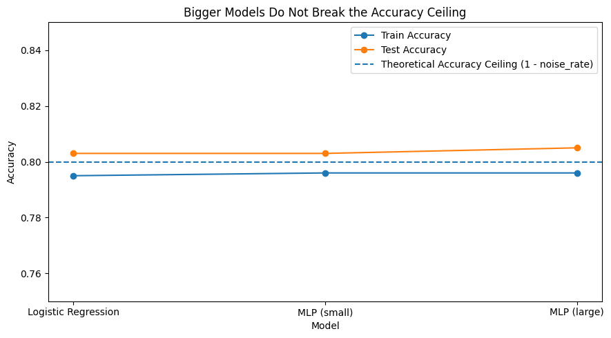
Results:

Model	Train Accuracy	Test Accuracy
Logistic Regression	0.795	0.803
MLP (small)	0.796	0.803
MLP (large)	0.796	0.805

Visualizing the Ceiling

As we increase model capacity, both training and test accuracy plateau at nearly the same level.

This tells us something important:

The model is not improving because there is no additional signal left to learn.

Model Capacity vs Train/Test Accuracy

Same Ceiling Across Models

Here, we keep the noise rate fixed at 20% and compare models with increasing capacity. The point is simple: once the information limit is reached, adding model capacity does not meaningfully improve performance.

import numpy as np
import matplotlib.pyplot as plt

from sklearn.model_selection import train_test_split
from sklearn.metrics import accuracy_score
from sklearn.linear_model import LogisticRegression
from sklearn.neural_network import MLPClassifier

np.random.seed(0)

n = 20000
noise_rate = 0.2

X = np.random.randn(n, 1)
y = (X[:, 0] > 0).astype(int)

flip = np.random.rand(n) < noise_rate
y[flip] = 1 - y[flip]

X_train, X_test, y_train, y_test = train_test_split(
    X, y, test_size=0.25, random_state=42
)

models = [
    ("LogReg", LogisticRegression()),
    ("MLP (5)", MLPClassifier(hidden_layer_sizes=(5,), max_iter=2000, random_state=42)),
    ("MLP (10)", MLPClassifier(hidden_layer_sizes=(10,), max_iter=2000, random_state=42)),
    ("MLP (50)", MLPClassifier(hidden_layer_sizes=(50,), max_iter=2000, random_state=42)),
    ("MLP (100,100)", MLPClassifier(hidden_layer_sizes=(100, 100), max_iter=2000, random_state=42)),
]

model_names = []
train_scores = []
test_scores = []

for name, model in models:
    model.fit(X_train, y_train)

    train_pred = model.predict(X_train)
    test_pred = model.predict(X_test)

    model_names.append(name)
    train_scores.append(accuracy_score(y_train, train_pred))
    test_scores.append(accuracy_score(y_test, test_pred))

plt.figure(figsize=(10, 5))
plt.plot(model_names, train_scores, marker="o", label="Train Accuracy")
plt.plot(model_names, test_scores, marker="o", label="Test Accuracy")
plt.axhline(y=1 - noise_rate, linestyle="--", label="Theoretical Ceiling")

plt.xlabel("Increasing Model Capacity")
plt.ylabel("Accuracy")
plt.title("More Capacity Does Not Break the Information Limit")
plt.ylim(0.75, 0.85)
plt.legend()
plt.tight_layout()
plt.show()

This is the point where the idea becomes hard to ignore. Across models, the achievable accuracy stays pinned near the same ceiling. The important thing is not that one model is slightly better than another. The important thing is that none of them escape the limit.

That is the signature of an information-limited problem. The ceiling doesn’t depend on the model - it depends on the noise.

Just like in the medical example, the model wasn’t failing because it was too simple. It was failing because data didn’t contain enough signal.

Why This is Not Underfitting or Overfitting

At this point, it’s natural to question what’s happening. If models are not improving, we usually fall back on the familiar explanations.

• Maybe the model is too simple (underfitting)
• Maybe it’s memorizing noise (overfitting)

But neither explanation fits what we’re seeing.

It’s not underfitting, because even simple models can learn the true rule.

It’s not overfitting, because training and test accuracy are close.

Instead:

The model is doing the best it possibly can given the information available.

The remaining errors are not due to bad optimization or insufficient model capacity. They exist because the data itself is uncertain.

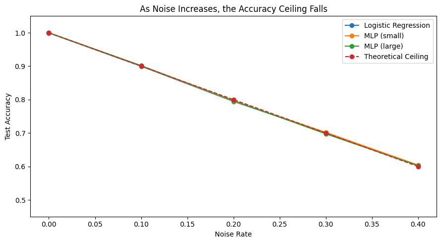
Why This Happens in Real ML Systems

So far, this was a controlled experiment. We deliberately injected noise to make the limit visible. But in real-world problems, no one tells you how much noise exists. And that’s where things get tricky.

In practice, when a model plateaus, the default reaction is almost automatic:

• Try a bigger model
• Tune hyperparameters
• Add more data
• Run more experiments

It feels like progress.

But often, it isn’t.

Because sometimes, the issue is not the model — it’s the amount of information available in the data.

Where does this “Noise” come from in reality?

In real systems, noise isn’t artificially injected. It comes from things you simply don’t observe.

For example:

• Churn prediction

  You can track clicks, sessions, and purchase history. But you cannot observe the moment a user simply loses interest, finds a better alternative, or goes through a life change that makes your product irrelevant. That decision happens entirely outside your data. No matter how much behavioral data you collect, the signal that actually drove the churn was never recorded.

• Medical diagnosis

  Two patients can present with identical symptoms, identical test results, and identical histories, and yet have different underlying conditions. Biology has individual variation that no standard set of features can fully account for. The ambiguity is not a gap in the data collection process. It is built into the problem itself.

In these cases, the data is inherently incomplete. The missing information is not something you can engineer your way around.

A Shift in Thinking

Instead of asking:

“How do I make the model better?”

You start asking:

“Do I have enough information to solve this problem?”

A More Useful Direction

When you hit this limit, the solution is not:

• bigger models
• more tuning

The solution is:

• better features
• better data
• better signals

In the end, models don’t create information - they extract it.

Conclusion: When the Limit Isn’t the Model

It’s easy to believe that better models should always lead to better results, and in many cases they do. But this experiment highlights something more fundamental: sometimes performance stops improving not because the model is weak, but because the problem itself has a limit. By creating a simple dataset and controlling the noise, we saw that increasing model capacity didn’t break the accuracy ceiling and that training and test performance plateaued together. That is the essence of Bayes Error: there is a limit to how well any model can perform, and that limit is set by the information available. In real-world systems, this limit is hidden. You don’t know the noise rate or exactly how much uncertainty exists; you only see a model that refuses to improve. And that’s where this perspective matters, because instead of endlessly tuning models, you can step back and ask a better question: am I trying to solve a problem that the data cannot fully answer? That shift changes how you approach machine learning. You stop chasing marginal gains through complexity and start focusing on improving the data itself.