Gradient Descent: The Never-Ending Quest for a Better Solution

By Rupesh on Jun 20, 2024

Gradient descent can be an intimidating topic, especially for beginners. It’s common to feel as if there’s a missing piece when trying to understand the inner workings of this robust optimization algorithm. In this blog, I aim to break down the topic into smaller, manageable fragments, presented in a sequence that makes it easier to grasp.

Introduction

In machine learning, the primary goal is to create a model that accurately predicts the output based on a given set of input data. However, there is often a difference between the actual value and the prediction made by the model. This discrepancy is quantified using a loss function, which measures the difference between the expected output and the actual output. The loss function is a crucial part of the optimization process, serving as an objective function for algorithms like gradient descent. Gradient descent is one of the simplest and most fundamental optimization algorithms used in machine learning to minimize the loss function. By reducing the loss function, the model’s predictions become closer to the actual values, resulting in improved performance.

Topics to understand beforehand

To fully comprehend gradient descent, a basic understanding of few topics is essential. It’s beneficial to explore these concepts individually before bringing them together in the context of gradient descent.

Optimization

Optimization is the process of finding the minimum or maximum value of a function. In machine learning, we often use optimization to train models. The goal is to determine the values of model parameters that minimize the error between the predicted value and the actual value. Effective optimization leads to better model performance and more accurate predictions.

Derivatives

Derivatives play a crucial role in gradient descent. They represent the slope of a function at a specific point. In the context of gradient descent, first-order derivatives are used to update the model’s parameters. By calculating the derivative, we can determine the direction and rate of change of the function, guiding us toward the minimum value of the loss function.

Gradient

The gradient of a function is the collection of partial derivatives in the form of a vector. The gradient of a function at a particular point is a vector that points in the direction of the maximum increase of the function. In other words, the gradient points in the direction of the steepest ascent.

Local minima and maxima

Local minima and maxima are points where a function attains its lowest or highest value within a small region. A local minimum is a point where the function value is lower than all nearby points, while a local maximum is higher than all nearby points. The global minimum, in contrast, is the absolute lowest value of the loss function across its entire domain. Understanding these concepts is crucial because gradient descent aims to find the global minimum, though it might sometimes get stuck in local minima.

How It Works

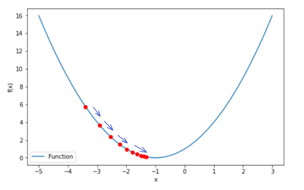
Gradient descent works by computing the gradient of the loss function with respect to model’s parameters. The gradient is a vector that points in the direction of the steepest increase/ascent in the function. By taking steps in the opposite direction of the gradient, we can move towards the minimum of the loss function. Finding the minimum of the loss function means that the predicted values are close to the actual values.

There is a formula to update the parameters in gradient descent. The formula is as follows:

X_{i+1} = X_i - \eta * \Delta J(X_i)

where $x_i$ is the vector of model parameters at iteration i, η is the learning rate and ∇J( $x_i$ ) is the gradient of the loss function with respect to $x_i$ .

The size of each step is determined by the learning rate, which is a hyperparameter that controls the step size. If the learning rate is too large, we may overshoot the minimum and fail to converge. If the learning rate is too small, we may take too long to converge.

Although gradient descent is a powerful algorithm, it has some limitations. One of the main challenges of gradient descent is finding the global minimum of the loss function. In some cases, the algorithm may converge to a local minimum instead of the global minimum, which can lead to suboptimal solutions. To address this issue, several techniques such as momentum-based gradient descent, adaptive learning rate methods, and stochastic gradient descent have been developed.

Convergence Criteria

It’s important to determine when to stop the iterations. Common criteria include:

Fixed Number of Iterations: Running the algorithm for a pre-determined number of steps.
Small Change in Loss Function: Stopping when the change in the loss function between iterations falls below a threshold.
Gradient Threshold: Stopping when the gradient becomes very small, indicating that further steps will not significantly reduce the loss.

Learning Rate Scheduling

Adjusting the learning rate during training can help achieve better performance. Techniques include:

Learning Rate Decay: Gradually reducing the learning rate as training progresses.
Adaptive Learning Rates: Using algorithms like Adam or RMSprop that adjust the learning rate based on the observed gradients.

Mathematical Example:

Suppose we have a quadratic function:

f(x) = x^2 - 4x + 4

The aim is to find the minimum of this function using gradient descent.

Step I: Compute the first derivative of the function

f'(x) = \frac{d}{dx}(x^2 - 4x + 4) = 2x - 4

Step II: Choose an initial point and learning rate

Suppose $x_0$ = 0 and learning rate η = 0.1

Step III: Iteratively update the parameter

Using the update rule:

x_{i+1} = x_i - \eta .f'(x_i)

Step IV: Step-by-Step iterations

Iteration 1:

$x_0$ = 0

$x_{i+1} = x_i - \eta .f'(x_i)$

$x_{0+1} = x_0 - 0.1* (2x_0 - 4)$

$x_{1} = 0 - 0.1* (2.0 - 4)$

$x_1$ = 0.4

Iteration 2:

$x_1$ = 0.4

$x_2$ = $x_1$ - $\eta$ . f’( $x_1$ )

$x_2 = 0.4 - 0.1 * (2 * 0.4 - 4)$

$x_2 = 0.72$

Similarly, $x_3$ = 0.976

The update rule is applied until $x_i$ converges to the minimum value.

Visualization of the Convergence; Image By Author

Conclusion

Gradient descent is a powerful optimization algorithm used to minimize a function by iteratively adjusting the input variables in the direction of the steepest decrease in the function. While it can be intimidating, with a basic understanding of calculus and optimization, and an appreciation for the concept of local minima and maxima, it becomes much more accessible. By iteratively adjusting model parameters in the direction of the gradient of the loss function, we can efficiently train machine learning models and improve their performance. Understanding its variants and enhancements, such as momentum, adaptive learning rates, and different types of gradient descent, further equips practitioners to tackle diverse optimization problems effectively.